suppressPackageStartupMessages({
  library("ape")           # For phylogenic data manipulation, plotting, etc.
  library("phangorn")      # Phylogenetic reconstruction, modeling, and analyses
})

# Function to select "Not In"
'%!in%' <- function(x,y)!('%in%'(x,y))

# read alignment
alignment <- read.dna("nepal_core_gene_alignment.aln", format = "fasta")
 
# make matrix for NJ tree and ML tree
dist_matrix <- dist.dna(alignment, model = "JC69")  # Jukes-Cantor distance model

First let’s try an unrooted tree, which allows you to see how your sequences are associated relative to each other, rather than to a common ancestor

Now let’s make a neighbor joining tree. Neighbor joining trees allow you to examine distances between sequences in terms of how many base pairs are changed between sequences, and builds a tree grouping the shortest possible distances

nj_tree <- nj(dist_matrix)
plot(nj_tree, main = "Neighbor Joining Tree", 
     cex = 0.6, edge.width = 2, font = 1)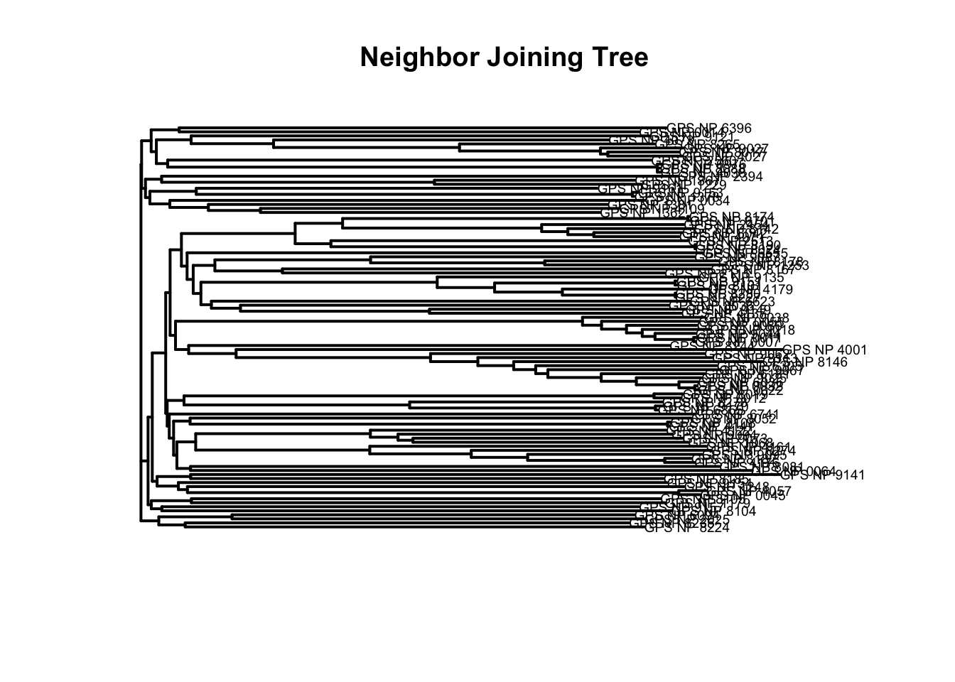

Now let’s try a maximum likelihood tree. Maximum likelihood trees use different modeling techniques, here the GTR, the General Time Reversible model which will use the overall frequncies of the bases and the frequency that they vary between sequences (e.g., all As, all Ts, all switches from A-T or T-A, )

Here we have the gamma parameter enabled which allows us to make heterogenous rates of evolution between different areas (some regions are conserved, some vary more) using a Gamma distribution.

phydat_alignment <- phyDat(alignment, type = "DNA")

# Start with NJ tree
start_tree <- nj(dist_matrix)

# Fit a model to examine rates of substitution (e.g. GTR + Gamma)
fit <- pml(start_tree, data = phydat_alignment)
fit <- optim.pml(fit, model = "GTR", optGamma = TRUE, control = pml.control(trace = 0))

only one rate class, ignored optGamma

fit$gamma  # here we can look at our different rates

NULL

# Plot ML tree
plot(fit$tree, main = "Maximum Likelihood Tree",
     cex = 0.6, edge.width = 2, font = 1)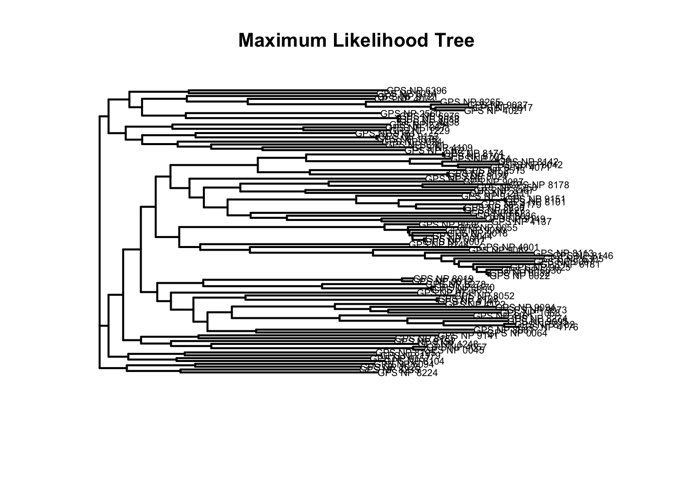

bootstrap consensus tree: randomly resamples your alignment and builds trees from each sample, then compares the trees and record the frequency of each branch across all trees. then it builds consensus tree that will contain all of the branches that occur in at least a given percentage of sample trees.

# boot_tree <- bootstrap.phyDat(alignment, FUN = function(x) optim.pml(pml(tree_nj, x), model = "GTR")$tree, bs = 10)
# cons_tree <- consensus(boot_tree, p = 0.5)#here is where you decide what percentage of trees need to contain the branch for it to appear in the consensus tree
# 
# plot(cons_tree, main = "Custom Bootstrap Consensus")

# # Step 6: Perform tree optimization
# fit <- optim.pml(fit, model = "JC", rearrangement = "stochastic")
# 
# # Step 7: Extract the ML tree
# ml_tree <- fit$tree
# 
# # Step 8: Ensure the tree is unrooted
# unrooted_ml_tree <- unroot(ml_tree)

# Read IQ-TREE .treefile (unrooted ML tree)
#tree_unrooted <- read.tree("example.treefile")
# plot(tree_unrooted, main = "Unrooted Tree", type = "unrooted")

#write.tree(nj_tree, file = "C:/nj_tree.nwk")
#write.tree(fit$tree, file = "C:/ml_tree.nwk")
#write.tree(boot_trees, file = "C:/boot_trees.nwk")

now we can take these over to Microreact!

Preset microreact dashboards: Malawi, Nepal, and Peru